Getting started

Installation

pyplotit is a pure python package, so the latest version can be installed with

pip install git+https://gitlab.cern.ch/cp3-cms/pyplotit.git

or, for an editable install when frequent updates and/or testing of changes is expected, with

git clone https://gitlab.cern.ch/cp3-cms/pyplotit.git
pip install -e ./pyplotit

Example: loading histograms from a plotIt configuration

If you do not have a plotIt configuration and the corresponding ROOT files around, you can use the following commands to generate an example; they are also used here for the rest of the example

!wget -q https://gitlab.cern.ch/cp3-cms/pyplotit/-/raw/master/tests/data/ex1_syst.yml
!wget -q https://raw.githubusercontent.com/cp3-llbb/plotIt/master/test/generate_files.C
!mkdir -p files
!root -l -b -q generate_files.C

We can load the configuration file ex1_syst.yml in pyplotit as follows:

import plotit
config, samples, plots, systematics, legend = plotit.loadFromYAML("ex1_syst.yml")

/home/docs/checkouts/readthedocs.org/user_builds/pyplotit/conda/latest/lib/python3.14/site-packages/cppyy_backend/loader.py:147: UserWarning: No precompiled header available (cannot import name 'get_cppversion' from 'cppyy_backend._get_cppflags' (/home/docs/checkouts/readthedocs.org/user_builds/pyplotit/conda/latest/lib/python3.14/site-packages/cppyy_backend/_get_cppflags.py)); this may impact performance.
  warnings.warn('No precompiled header available (%s); this may impact performance.' % msg)
C system headers (glibc/Xcode/Windows SDK) must be installed.
In file included from input_line_4:36:
/home/docs/checkouts/readthedocs.org/user_builds/pyplotit/conda/latest/bin/../lib/gcc/x86_64-conda-linux-gnu/14.3.0/include/c++/cassert:44:10: fatal error: 'assert.h' file not found
#include <assert.h>
         ^~~~~~~~~~

Most of the returned objects are either (lists of) simple objects that represent a part of the configuration, e.g. a single plot. The classes are implemented as data classes. The list returned in samples is based on the entries in the files block of the configuration file, but using the grouping specified by their group attributes and the list of groups, such that each entry corresponds to a visible contribution in the plots.

Since the File and Group classes also contain functionality for the efficient loading and summing of the histograms, the pure configuration part is kept in a separate class (also a data class), under the cfg attribute. For groups the list of grouped files can be found under files.

[smp.cfg for smp in samples]

[File(type='MC', name='MC_sample2.root', order=0, legend='MC 2', legend_style='lf', legend_order=0, drawing_options='', marker_size=None, marker_color=None, marker_type=None, fill_color='#53777A', fill_type=1001, line_width=0, line_color=(0.0, 0.0, 0.0, 1.0), line_type=None, era=None, group=None, cross_section=666.3, branching_ratio=1.0, generated_events=2404, scale=1.0, pretty_name='MC_sample2.root', yields_title=None, yields_group='MC 2', legend_group=None),
 File(type='DATA', name='data.root', order=None, legend='Data', legend_style=None, legend_order=0, drawing_options='', marker_size=1, marker_color=(0.0, 0.0, 0.0, 1.0), marker_type=20, fill_color=None, fill_type=None, line_width=1, line_color=None, line_type=None, era=None, group=None, cross_section=1.0, branching_ratio=1.0, generated_events=1.0, scale=1.0, pretty_name='data.root', yields_title=None, yields_group='Data', legend_group=None),
 File(type='MC', name='MC_sample1.root', order=1, legend='MC 1', legend_style='lf', legend_order=0, drawing_options='', marker_size=None, marker_color=None, marker_type=None, fill_color='#D95B43', fill_type=1001, line_width=0, line_color=(0.0, 0.0, 0.0, 1.0), line_type=None, era=None, group=None, cross_section=245.8, branching_ratio=1.0, generated_events=2167, scale=1.0, pretty_name='MC_sample1.root', yields_title=None, yields_group='MC 1', legend_group=None)]

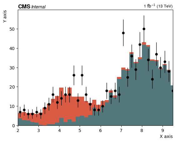
Typical plots contain an observed histogram and expectation stack. Since the former may be the sum of multiple datasets, it is also handled as a stack:

p = plots[0]
from plotit.plotit import Stack
expStack = Stack([smp.getHist(p) for smp in samples if smp.cfg.type == "MC"])
obsStack = Stack([smp.getHist(p) for smp in samples if smp.cfg.type == "DATA"])

The above works because both the File and Group class have a getHist method, which loads a single histogram from a file, or triggers the loading of multiple histograms and adds them up, respectively.

getHist returns a small object similar to a smart pointer: for a single file it holds the pointer to the (Py)ROOT histogram, for a group of stack it lazily constructs the sum histogram, or adds up the contents and squared weights arrays, depending on which method is called (more details will be added once the interfaces are more stable). These smart pointer or histogram handle classes also implement the uhi PlottableHistogram protocol, so they can directly be used with e.g. mplhep:

from matplotlib import pyplot as plt
fig, ax = plt.subplots()
ax.set_xlim(*p.x_axis_range)
import mplhep
mplhep.histplot(obsStack, histtype="errorbar", color="k")
mplhep.histplot(expStack.entries, stack=True, histtype="fill", color=[e.style.fill_color for e in expStack.entries])
ax.set_xlabel(p.x_axis, loc="right")
ax.set_ylabel(p.y_axis, loc="top")
mplhep.cms.label(data=True, label="Internal", lumi=config.getLumi())

/home/docs/checkouts/readthedocs.org/user_builds/pyplotit/conda/latest/lib/python3.14/site-packages/mplhep/utils.py:741: UserWarning: Integer weights indicate poissonian data. Will calculate Garwood interval if ``scipy`` is installed. Otherwise errors will be set to ``sqrt(w2)``.
  self.errors()

(exptext: Custom Text(0.0, 1, 'CMS'),
 expsuffix: Custom Text(0.0, 1.005, 'Internal'),
 supptext: Custom Text(1.012, 1, ''))